December 21, 2022 · 9 min read
Adversarial Examples

Today I’m glad to introduce you to one of my favorite topics, the “adversarial examples”
Adversarial machine learning
As cyber-security is the practice of attacking and protecting computing systems from digital attacks, adversarial machine learning (AML) is the study of the attacks on machine learning algorithms and the defenses against such attacks.
These attacks can target different types of Machine Learning (ML) systems, such as escaping spam filters by obfuscating spam messages, misleading an intrusion detection system (IDS) by modifying the characteristics of a network flow or even leading an autonomous car to misinterpret a stop sign for a speed limit sign.
AML techniques can target different parts of the model flow by applying evasion attacks, model extraction, or even generating adversarial examples. In this article, we will focus on the last one, the generation of adversarial examples.
Adversarial Examples
An adversarial example is a specially crafted input designed to look “normal” to humans but causes misclassification to a ML model.
Adversarial example attacks can be targeted or untargeted. As the name suggests, targeted attacks have a target class that it wants the target model to predict, whereas untargeted attacks only aim to cause misclassification to the ML model. Untargeted attacks tend to be faster compared to targeted where targeted tend to produce better results.
Adversarial examples can be subdivided into White box attacks and Black box attacks. Let’s see their difference and how they each work.
White box attacks
White box attacks assume that you have access to the target model. It’s rarely the case in real-world situations but they lay the foundations of black-box attacks; thus, it’s essential to understand how they work.
Let’s rewind to the training process of ML models, minimizing the determined loss function that works as a criterion for the model.
This can be written as:
Repeating the back-prop, the model starts converging to a suitable set of parameters. This training process works because, at each training iteration, we calculate the gradient of the loss function with respect to all the weights in the network to know how to modify it.
What if, instead of modifying the model’s parameters to minimize the loss function, we modify the model’s input to maximize the loss function? That’s precisely the mean idea behind the adversarial examples!
FGSM

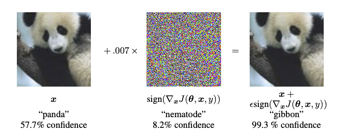
The fast gradient sign method (FGSM) introduced by Ian J. Goodfellow, Jonathon Shlens, and Christian Szegedy in Explaining and Harnessing Adversarial Examples works by using the gradients of the neural network to create an adversarial example.
The FSGM aims to find how much each pixel in the image contributes to the loss value and to add a perturbation to it accordingly.
To know which pixels to modify, FGSM uses the gradients of the loss with respect to the input image to create a mask that maximizes the loss. We then add this mask to our original image resulting in the adversarial image. To ensure the adversarial image is indistinguishable from the original image, we use a factor that controls how much we apply the produced mask to the original image.
We can summarize this process as follows:
Where:
- : Adversarial image.
- : Original input image.
- : Original input label.
- : Multiplier to ensure the perturbations are small.
- : Model parameters.
- : Loss
BIM
The basic iterative method (BIM, aka Iterative FGSM or I-FGSM) introduced in Adversarial examples in the physical world by Alexey Kurakin, Ian J. Goodfellow, and Samy Bengio is an extends the idea of the FGSM by applying perturbations iteratively with small steps size.
Applying perturbations has one main benefit over a one-shot method; as you modify the original input data in small steps, we ensure the generated adversarial example is closer to the original input data. On the other hand, the counter benefit is that it requires more steps and thus is computation more expensive.

BIM can be summarized as follows:
Where:
- : Adversarial image at step N
- : Original input image.
- : Original input label.
- : Multiplier to ensure the perturbations are small.
- : Clip factor to limit the perturbations at each step.
- : Model parameters.
- : Loss

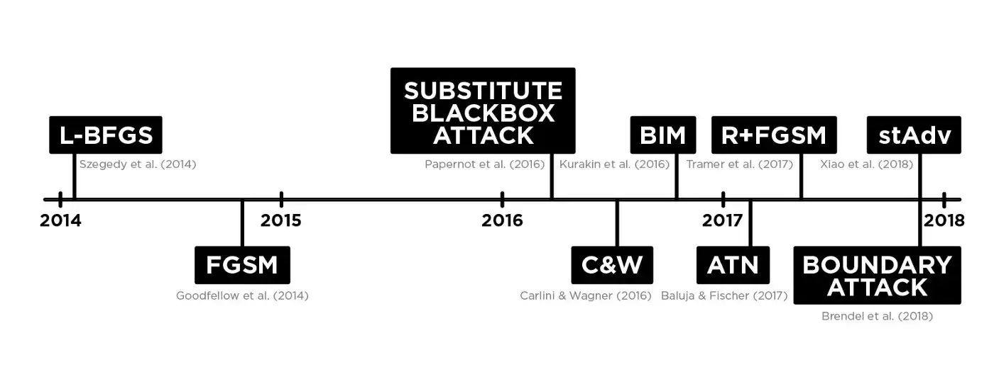
There are multiple other techniques to produce adversarial examples (L-BFGS, C&W, R+FGSM) that I would love to cover, but I try to keep those posts quick and straightforward to read.
Note:Feel free to let me know in the comments if you prefer more in-depth articles for the future.
So without waiting any further, let’s dive into the black box techniques for adversarial examples!
Black box attacks
Some of you might think “Okay adversarial examples are cool, but in practice, the attacker will not have access to the model’s parameters, so we’re safe, right?”.
Indeed for those attacks to work, we need to have access to the model parameters, but what if we don’t have access to those parameters? Well, we can try to recreate it!
Transferability of adversarial examples
Imagine you have a model M trained to classify the MNIST dataset but need access. The attacker could create a substitute model S, also trained on MNIST, that it would use to create his adversarial examples and then send it to the target model M. Does it work? Yes, thanks to the notion of transferability of adversarial examples.
We could summarize those steps as follows:
- A target model M is trained, and its parameters are unknown to the attacker.
- A substitue model S is trained to mimic the target model M.
- An adversarial example is generated using model S.
- The generated adversarial example is applied to model M thanks to the notion of transferability of adversarial examples

The most attentive among you might say “Okay then, but what if we don’t have access to the dataset used to train the model?”. To that, I will respond, what if we could guess the original dataset used to train the model?
Membership Inference Attacks
A model is served on a cloud (GCP, Azure ML, AWS, or whatever), the attacker doesn’t have access to either the model or the cloud; it can only query the model and retrieve its raw prediction (in case of a classifier, its confidence scores). In this case, we might think that it’s safe to say our model is well protected, and the attacker won’t be able to either reproduce the model or the dataset it was trained on.
This is where the membership inference attacks come in place!
The main goal of the membership inference attacks is to determine whether input data is issued from the target model’s training set. In that goal, we will create an attack model to apply a binary classification on the input data predicting if it’s present in the target model’s training set.
Now the question is how to get the necessary data to train such a model. For that, we will need what is called “Shadow models”; shadow models imitate the target model. They need to be of the same type and have the same architecture as the target model, but obviously, their parameters will be different.

Those shadow models need to be trained too, and once again comes the question of the training data. How to train those shadow models? Here we have two options :
1 - Real data
Here, we know the data distribution of the target model; thus, we have to collect data from the data distribution to generate our training set.
2 - Synthetic data
In real-world cases, the attacker probably won’t know nor have access to the used data distribution. The attacker will have to generate a synthetic dataset by following the following steps:
- Attacker create random input data (noise)
- Attacker provides this data to the target model
- Attacker uses a search algorithm to update the provided input data
- Repeat steps 1-3 until a sufficient dataset is generated.
Attackers can now train their attack model, use it to generate the target model’s training set, develop its model, and finally create adversarial examples. In practice, this process is expensive and time-consuming, demonstrating the vulnerability of deployed ML models, even in a black-box context. Another limitation is that it is too costly to re-train those models with a large model, thus preventing the attacker from re-creating its substitute model to generate adversarial examples.
Side note 1 : It exists techniques to limitate the number of input data to retrieve such as the Jacobian-based dataset augmentation technique?
Side note 2 : I recommend this great video by IEEE Symposium on Security and Privacy that explain more in details how the Membership Inference Attacks work.
Conclusion
As we’ve seen, adversarial examples are a pretty straightforward method to attack machine learning models while still being undetectable in the first view by a human.
It exists a multitude of other attacks for generating adversarial examples both in a white box context (L-BFGS, C&W, …) and a black box context (Boundary Attack, Zeroth-order optimization attack (ZOO) …), each with pros and cons. If you want to try some of those attacks, I invite you to test OpenAdv, a project I made while discovering adversarial attacks in 2021.
I like to present in another blog post techniques to protect our model against adversarial attacks; feel free to let me know if you find it interesting or if you have another topic you would like to be covered.
You can find me on Github, Twitter, and LinkedIn, feel free to reach me, it’s always a pleasure to discuss with passionate people.